In the previous section, we discussed how to calculate node purity for classification and regression trees. However, two important questions remain unanswered:

• How does the algorithm determine the threshold for the variable split?
• How does the algorithm decide which variable to select for splitting?

In this section, we will discuss information gain, which will help us understand these questions.

Information Gain

As discussed earlier, a decision tree splits data in a way that makes the partitions more homogeneous. When the algorithm splits a variable at a particular threshold, information gain helps determine whether the resulting partitions have become more homogeneous. If they have, the split is accepted; otherwise, the algorithm rejects the split and tries a different threshold.

Information gain is defined as the difference between node purity before and after the split.

Calculation of Information Gain

Consider the example tree shown in the diagram below. Assume this represents the current state of the tree.

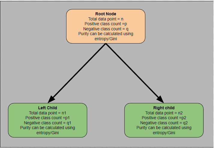
The root node contains p positive class and q negative class data points. We can calculate the root node purity using either entropy or Gini impurity, depending on our choice. Let's denote this impurity as \( G(\text{root}) \), which represents the impurity before the split.

• Impurity Before Split

  Total number of data points: n
  Count of positive class: p
  Count of negative class: q
  Probability of class 0: \( p_0 = \frac{q}{n} \)
  Probability of class 1: \( p_1 = \frac{p}{n} \)
  Entropy before split: \[ \text{Entropy}_{\text{before split}} = -p_0 \log (p_0) - p_1 \log (p_1) \]

• Impurity After Split

  When the selected variable is split at a given threshold, it creates left and right child nodes. To calculate impurity after the split, we compute the impurity for both child nodes and take their weighted average.

  • Entropy for Left Child Node

    Total number of data points: \( n_1 \)
    Count of positive class: \( p_1 \)
    Count of negative class: \( q_1 \)
    Probability of class 0: \( p_0 = \frac{q_1}{n_1} \)
    Probability of class 1: \( p_1 = \frac{p_1}{n_1} \)
    Entropy for the left child: \[ \text{Entropy}_{\text{left}} = -p_0 \log (p_0) - p_1 \log (p_1) \]

  • Entropy for Right Child Node

    Total number of data points: \( n_2 \)
    Count of positive class: \( p_2 \)
    Count of negative class: \( q_2 \)
    Probability of class 0: \( p_0 = \frac{q_2}{n_2} \)
    Probability of class 1: \( p_1 = \frac{p_2}{n_2} \)
    Entropy for the right child: \[ \text{Entropy}_{\text{right}} = -p_0 \log (p_0) - p_1 \log (p_1) \]

  The entropy after the split is calculated as the weighted average of the left and right child entropies:

  Weight for left child: \( w_{\text{left}} = \frac{n_1}{n_1 + n_2} \)
  Weight for right child: \( w_{\text{right}} = \frac{n_2}{n_1 + n_2} \)
  

  \[ \text{Entropy}_{\text{after split}} = w_{\text{left}} \cdot \text{Entropy}_{\text{left}} + w_{\text{right}} \cdot \text{Entropy}_{\text{right}} \]

Finally, information gain is calculated as:

\[ \text{Information Gain} = \frac{n}{N_{\text{total}}} \cdot (\text{Entropy}_{\text{before split}} - \text{Entropy}_{\text{after split}}) \]

Where \( N_{\text{total}} \) is the total number of data points in the entire dataset.

In the above explanation, we calculated information gain using entropy. However, we can also use Gini impurity to compute information gain for classification trees. For regression trees, entropy/Gini is replaced with variance, while the rest of the calculation remains the same.