Introduction

A Decision Tree is a supervised learning algorithm that can be used for both classification and regression tasks. We have already explored linear regression for regression tasks and logistic regression for classification tasks. So, why do we need another algorithm for these problems?
Linear and logistic regression are simple algorithms that can learn linear patterns in data. However, they are ineffective when dealing with non-linear patterns. Therefore, we need algorithms that can effectively capture non-linear patterns.
The Decision Tree algorithm is one such approach that can model non-linear patterns in data. It works by partitioning the data into segments, ensuring that each segment becomes more homogeneous. The majority of data points in a given partition exhibit similar characteristics.
Consider an example where we aim to predict whether a customer will default on a loan based on their income and risk score. The scatter plot in Figure 1 visualizes this data. Green points represent customers who did not default (good customers), while orange points indicate customers who defaulted (bad customers).
Clearly, a single linear boundary cannot effectively separate the green and orange points, indicating that the decision boundary is non-linear.

To distinguish between good and bad customers, we can create decision boundaries by selecting a variable and splitting it at a certain threshold.
In our example, we first split based on the income variable, followed by a split using the risk variable. Two key questions arise:

1. Which variable should be selected for splitting?
2. How do we determine the optimal split threshold?

We will explore these questions later in the discussion For now, let's see how feature space partitioning makes the data more homogeneous, giving us a high-level overview of how the Decision Tree algorithm works.

Split 1: Is income >= 14.5?

The black line represents the decision boundary (income = 14.5). The region below the boundary (red region) has become homogeneous, consisting primarily of customers who defaulted on their loans.
The region above the boundary (green region) remains heterogeneous, containing both positive and negative class data points, requiring further splitting.

Split 2: Given income >= 14.5, is risk_score < 95?

The green region still contains a mixture of positive and negative class data points. Therefore, we further split it into a third region (light blue). The blue line represents the decision boundary (risk_score = 95).

Now, we have a total of three regions, each of which is homogeneous. We can compute the probability of default in each region:

• Region 1: income < 14.5 (Red Region)
  10 orange points (default), 1 green point (non-default)
  \( p(\text{default}) = \frac{10}{11} \)


• Region 2: income >= 14.5 and risk_score < 95 (Green Region)
  2 orange points, 15 green points
  \( p(\text{default}) = \frac{2}{17} \)


• Region 3: income >= 14.5 and risk_score >= 95 (Blue Region)
  4 orange points, 0 green points
  \( p(\text{default}) = \frac{4}{4} \)
  

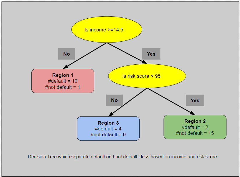
Constructing the Final Decision Tree

By splitting variables at optimal thresholds, we have divided our feature space into three distinct regions. Using this information, we can now construct the final Decision Tree, as shown in the figure below. Each region corresponds to a leaf node in the Decision Tree.