What will you learn in this section
- We will explore Assumptions of Linear Regression Model
- We will learn how to diagnose problems in the model
Once we have trained the model we need to check for potential problems in the model.
The Linear Regression Model has some inbuilt assumptions. These assumptions can be leveraged as
a diagnostic tool for Linear Regression models. If the trained model satisfied all of the assumptions
then the model is ready for use otherwise we need to make changes in our model.
In this section we will look at the following
- Important Assumptions in the Linear regression model
- How to check if assumptions are satisfied by trained model
- What steps one should take if any of the assumptions is not satisfied
1. Linearity of response-predictor relationship
Linear relationships between dependent and independent variables should exist. If there exists a non-linear
relationship between them then a trained model may not be a good model. We need to fix this issue and if we
are unable to fix this then we might have to use some non-linear regression approach.
How to check if assumption of linear relationship holds true or not?
Below are the ways to check this1. Scatter plot using independent and dependent variables
We can create a scatter plot between independent variable and dependent variable, and then through visual inspection we can determine if the relationship is linear or not.This approach is not scalable. We can use this approach only when we have fewer independent variables. As the number of independent variables increases this approach may be time consuming.
2. Residual Plots
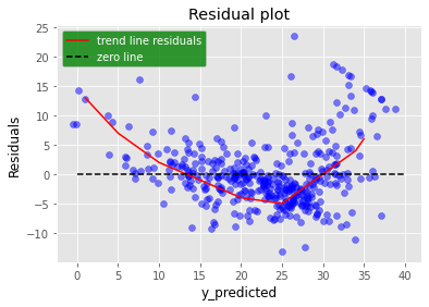
We can plot residuals \( (y_i-\hat{y_i}) \) vs predicted values \( \hat {y_i} \). If any of the patterns can be observed in this plot then it means Linearity assumption is violated. If the plot is completely random around a zero residual line then it means linearity criteria is satisfied.Below figure shows one example residual plot. You can clearly see the pattern in the plot which is highlighted by a red line. This means the trained model is violating the linearity assumption.
What steps should we take if linearity assumption is violated
There could be many ways to solve this issue. One of the possible ways is to apply non linear transformations such as \( \log (X), \sqrt X \ etc \) on independent variables and then re-train your model with transformed data and perform the same analysis with the updated model.2. Homoscedasticity : Constant variance of error terms
This means variance of residuals should be independent of response variable. Sometimes variance in residuals increases
as dependent variable value goes up. If variance of residuals is a function of y then this phenomenon is called
heteroscedasticity.
How to check this assumption
Create a residual plot and if a funnel type pattern is observed in the residual plot then it means variance of residuals is non constant. Below plot shows this behavior where variance in residuals increases as y predicted increases.
How to resolve this issue
In this case we can apply some transformation on the dependent variable to suppress its variance. \( \log(y), \sqrt(y)\) are few examples of such transformation. Larger values of y are more suppressed as compared to smaller y values. And hence smaller residuals for larger y values.3. Non-collinear independent variables
Collinearity means any pair of the independent variables are correlated with each other. Linear regression assumes no pair of independent variables should be correlated. Because of collinearity we have a very serious problem in model interpretation. Model parameters associated with collinear variables are very unstable. If we re-train our model with the same hyperparameters and same data you might get very different coefficients associated with collinear variables. Although you may get similar model performance in terms of standard error. Let's say we have a linear model with two variables. Let's assume bais term is zero ( just for simplicity) \begin{align} \\ \hat{y}&=a_1*x_1+a_2*x_2 \\ \\ error &=\frac{\sum_{i=1}^N(y_i-\hat{y_i})^2}{2*N} \end{align} linear regression tries to find \( a_1,a_2\) such that \(error\) is minimized. We can plot the contour map of \( error\) on the \(2D\) plane. Below figure shows contour plot of cost function for two cases
a. If \( x_1,x_2 \) are non collinear
In this case contours are circular in shape. Balck point shows the convergence point where error is minimum. Model re-training will produce \( a_1,a_2 \) values somewhere in the red band region. \( a_1 \in [4.7,5.3] \ , \ a_2 \in [4.7,5.3] \).b. If \( x_1,x_2\) are collinear
In this we get elongated contours. Black point shows the point of convergence. Model re-training will produce \(a_1,a_2 \) values somewhere in the red band region.\( a_1 \in [3.5,6.5] \ , \ a_2 \in [3.5,6.5] \). In this case model parameters lie in a bigger interval. Hence the model becomes a little bit unstable. On re-training you will get significantly different \( a_1, a_2 \) values but error measurement in both cases will be very close.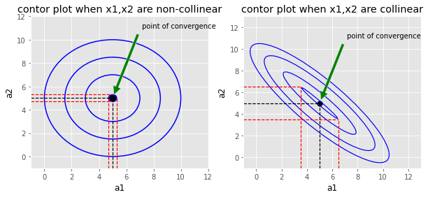
How to identify multi-collinearity
We can calculate correlation matrix of the independent variables and check if any pair of variables have significantly high correlation.Another way of identifying collinearity is by calculating the variance inflation factor (VIF). VIF value closer to 1 indicates no multicollinearity and VIF values in the range of 5 to 10 indicate problematic collinearity.
How to resolve this
- Remove one of the variables from the correlated pair.
- Take the ratio of variables and use the new variable instead of using the individual variables.
4. Un-correlated error terms
It means for any data point \((x_i,y_i)\), the error term should not give any information about the error of \( (i-1) th \ or \ (i+1) th \) data point. They should be completely independent of each other. If error terms are correlated then it leads to underestimation of standard error. Confidence intervals of parameters and p-values are dependent on standard error therefore they are also affected.[Add link related to confidence interval]