What You Will Learn in This Section
- How to define the mathematical model for Linear Regression
- Understanding the Least Squares error function
- Fundamentals of optimization algorithms
First, we will explore the key components of the Linear Regression algorithm. Then, we will combine these components to understand the complete algorithm. Generally, machine learning algorithms consist of three main components:
- Model
- Cost Function
- Optimizer
Let's examine these components in the context of Linear Regression.
1. Model
The model defines the relationship between the dependent variable (\(y\)) and the independent variable (\(x\)). Different machine learning algorithms use different models. The house price prediction equation from the previous section is an example of a linear model. For simplicity, we will first define our model using a single variable and later extend it to multiple variables. The Linear Regression model is represented by Equation 1:
Here, \(a_1\) and \(b\) are the model parameters, which we will learn to calculate in the next section. The notation \(\hat{y_i}\) represents the predicted \(y\) value for a given \(x\).
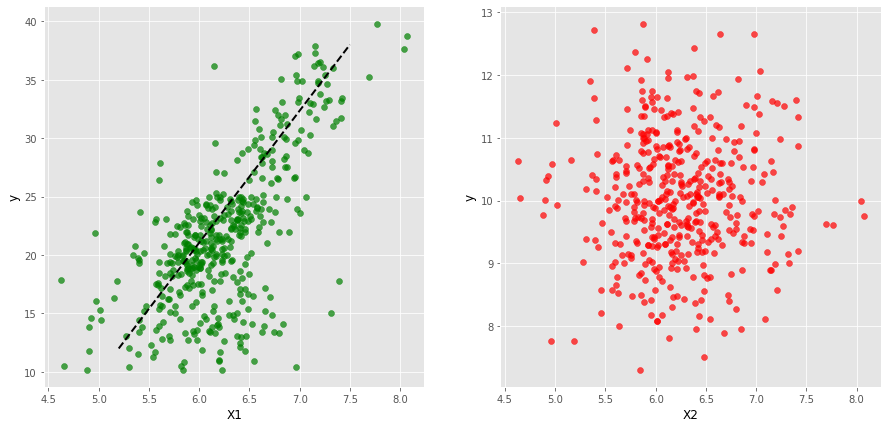
When defining a model, we must ensure that the independent variable (\(x\)) contains relevant information about the dependent variable (\(y\)). This can be understood through visualization. In the diagram below, the left plot shows a strong linear relationship between \(x_1\) and \(y\), whereas the right plot appears random, indicating no linear relationship between \(x_2\) and \(y\). Hence, it is more appropriate to use \(x_1\) to define a linear model rather than \(x_2\).
2. Cost Function
The cost function measures how close the predicted values are to the actual values of the dependent variable. The model equation provides the predicted value (\(\hat{y}\)), while the actual value (\(y\)) comes from the dataset. The error is defined as the difference between these two values. In Linear Regression, we use the squared error cost function:
Equation (3) is derived by substituting the value of \(\hat{y_i}\) from Equation 1. Here, \(a_1\) and \(b\) are the parameters, while \(x_i\) and \(y_i\) come from the data. The cost function can be represented as:
\[ J(a_1, b) = \frac{1}{2N} \sum_{i=1}^{N} ( y_i - a_1 x_i - b )^2 \]This error function is known as the Least Squares Cost Function.
The equation above shows that the average error is a function of the model parameters \(a_1\) and \(b\). The Linear Regression algorithm determines these parameters in such a way that the average error is minimized.
3. Optimizer
The optimizer helps determine the optimal values of parameters \(a_1\) and \(b\) to minimize the overall error. Let's develop an intuitive understanding of how optimization works:
If we examine the cost function equation, we observe that the only unknowns are the model parameters \(a_1\) and \(b\). Other elements, such as \(x_i\) and \(y_i\), are known data points, and \(N\) represents the total number of data points.
The optimizer starts by choosing initial values for \(a_1\) and \(b\) (let's pick, \(a_1=0\), \(b=25\)). It then calculates the cost function using these initial values. Subsequently, it updates the parameter values, taking steps in the direction that reduces the cost function. This process continues until the error is minimized.
The diagram below illustrates this process. The left plot shows the initial step with \(a_1=0\) and \(b=25\), where the fitted line is horizontal, resulting in a high cost function value. The middle plot demonstrates some improvement in the fit, while the right plot represents the best-fitted line. As the line improves, the cost function value decreases. The red lines indicate residuals, representing the difference between the actual and predicted values for each data point.
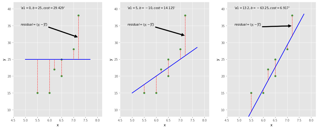
The optimization algorithm discussed above is called Gradient Descent.
Summary of This Chapter
- We first defined a model to calculate the predicted \(y\) values.
- We then examined the squared cost function, also known as the objective function or loss function.
- Finally, we explored how the optimizer leverages both the model and cost function to compute optimal model parameters.