Learning Curve

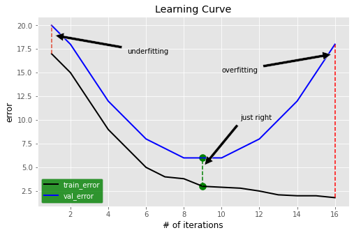
During model training, we can monitor performance using a cost function, error metric, or any other relevant measure on both training and validation datasets. Generally, the training error decreases as training progresses. However, if the validation error starts increasing after a certain point, you need to be cautious. The plot below illustrates how the error varies with the number of iterations for training and validation datasets. Three key scenarios are highlighted:

• Underfitting
  

  When both the training and validation errors are high and close to each other, it indicates that the model has not been trained sufficiently. This scenario is also known as high bias.

• Overfitting
  

  When the training error is low, but the validation error is significantly higher, the model is said to be overfitting. In this case, the model performs well on the training dataset but fails to generalize to unseen data (validation dataset). This is not desirable and is referred to as a high variance problem. We will explore ways to mitigate overfitting in different scenarios.

• Optimal Fit
  

  At this point, both training and validation errors are relatively low and close to each other. This indicates that the model generalizes well on both the training and validation datasets. Ideally, we aim for a model with low bias and low variance, but in practice, finding a good trade-off between the two is crucial.

Regularization: A Solution to Overfitting

There are multiple ways to address overfitting, and one of the most commonly used techniques is regularization. Regularization applies a penalty to model parameters through the cost function by adding an additional term. Let's examine the modified cost function.

Cost function without regularization
\begin{align} J(a_1,a_2...a_k,b)&=\frac{\sum_{i=1}^N \ (y_i-a_1*x_1-a_2*x_2......-a_k*x_k-b)^2}{2*N} \\ \end{align}

Cost function with \(L2\) regularization
\begin{align} J(a_1,a_2...a_k,b)&=\frac{\sum_{i=1}^N \ (y_i-a_1*x_1-a_2*x_2...-a_k*x_k-b)^2}{2*N} \ + \frac{\lambda*(a_1^2+a_2^2...a_k^2)}{2*N} \\ \end{align} Here, \( \lambda \) is the regularization parameter.
Typically, we do not regularize the bias term. This particular approach is called \(L2\) regularization. A similar method, known as \(L1\) regularization, uses the absolute values of parameters instead of squaring them.

Cost function with \(L1\) regularization
\begin{align} J(a_1,a_2...a_k,b)&=\frac{\sum_{i=1}^N \ (y_i-a_1*x_1-a_2*x_2...-a_k*x_k-b)^2}{2*N} \ + \frac{\lambda*(|a_1|+|a_2|...|a_k|)}{2*N} \end{align} For now, we will focus on \( L2 \) regularization. Since the cost function has changed, the gradients of the cost function with respect to the parameters will also change: \begin{align} \partial a_1 &=\frac{\sum_{i=1}^N \ (y_i-\hat{y_i})*(-x_{1i})}{N} \ + \frac{\lambda *a_1}{N}\\ \partial a_2 &=\frac{\sum_{i=1}^N \ (y_i-\hat{y_i})*(-x_{2i})}{N} \ + \frac{\lambda *a_2}{N} \\ .\\ .\\ .\\ \partial a_k &=\frac{\sum_{i=1}^N \ (y_i-\hat{y_i})*(-x_{ki})}{N} \ + \frac{\lambda *a_k}{N} \\ \partial b &=\frac{\sum_{i=1}^N \ (y_i-\hat{y_i})*(-b)}{N} \\ \end{align} These updated gradient values are used to update the model parameters during optimization.

\( L2 \) Regularization is also called Weight Decay Regularization

To understand why, let's analyze the gradient equation after introducing the regularization term in the cost function: \begin{align} \partial a_1 &=\frac{\sum_{i=1}^N \ (y_i-\hat{y_i})*(-x_{1i})}{N} \ + \frac{\lambda *a_1}{N} \end{align} Looking at the right-hand side of the equation, the first term represents the gradient value without regularization. We can rewrite it as: \begin{align} \partial a_1 = \partial a_1 (no \ reg) + \frac{\lambda *a_1}{N} \end{align} Now, considering the parameter update equation: \begin{align} a_1 &= a_1 - \alpha *\partial a_1 \\ a_1 &= a_1 - \alpha * \{ \partial a_1 (no \ reg) + \frac{\lambda *a_1}{N} \} \\ a_1 &= a_1 - \alpha * \partial a_1 (no \ reg) - \frac{\alpha * \lambda a_1}{N} \\ a_1 &= a_1 ( 1-\frac{\alpha * \lambda}{N}) - \alpha * \partial a_1(no \ reg ) \end{align} The first term on the right-hand side introduces a small decay before the actual update occurs. Due to this decay effect, \( L2 \) regularization is often referred to as weight decay regularization.